November 29, 2012

Some Good Advices


There's some fine advice.

Give people more than they expect and do it cheerfully. 

Marry a man/woman you love to talk to. As you get older, their conversational skills will be as important as any other.. 

Don't believe all you hear, spend all you have or sleep all you want. 

When you say, "I love you," mean it. 

When you say, "I'm sorry," look the person in the eye. 

Be engaged at least six months before you get married. 

Believe in love at first sight. 

Never laugh at anyone's dream. People who don't have dreams don't have much. 

Love deeply and passionately. You might get hurt but it's the only way to live life completely. 

In disagreements, fight fairly. No name calling. 

Don't judge people by their relatives. 

Talk slowly but think quickly. 

When someone asks you a question you don't want to answer, smile and ask, "Why do you want to know?" 

Remember that great love and great achievements involve great risk. 

Say "God bless you" when you hear someone sneeze. 

When you lose, don't lose the lesson  

Remember the three R's: Respect for self; Respect for others; and responsibility for all your actions. 

Don't let a little dispute injure a great friendship. 

When you realize you've made a mistake, take immediate steps to correct it. 


Smile when picking up the phone. The caller will hear it in your voice. 

Spend some time alone.


Heavy rains remind us of challenges in life. Never ask for lighter rain.  Just pray for a  better umbrella. That is attitude.

When flood comes, fish eat ants & when flood recedes, ants eat fish. 
Only time matters. Just hold on, God gives an opportunity to everyone!

Life is not about finding the right person, but creating the right relationship, it is not how we care in the beginning, but how much we care till the end.

 Some people always throw stones in your path. It depends on you what you make with them. Wall or Bridge?  Remember you are the architect of  your life.

Every problem has (n+1) solutions, where n is the number of solutions that you have tried and 1 is that which you have not tried. That's life.

Search a beautiful heart, but do not search for a beautiful face. Since beautiful things are not always good, but good things are always beautiful.

It's not important to hold all the good cards in life. But it is
important how well you play with the cards that you hold.

Often when we lose all hope & think this is the end, God smiles from above and says: "relax dear its just a bend. Not the end".
When you feel sad, to cheer up just go to the mirror and say: "Damn I am so cute" and you will overcome your sadness. But do not make this  a habit because liars go to hell :)

One of the basic differences between God and human is, God gives, gives and forgives. But human gets, gets, gets and forgets.

November 23, 2012

Complete Binary Tree

We have earlier discussed the properties of the binary trees besides talking about the internal and external nodes’ theorem. Now we will discuss another property of binary trees that is related to its storage before dilating upon the complete binary tree and the heap abstract data type.
Here is the definition of a complete binary tree:
  • A complete binary tree is a tree that is completely filled, with the possible exception of the bottom level.
  • The bottom level is filled from left to right.
A binary tree T with n levels is complete if all levels except possibly the last are completely full,
and the last level has all its nodes to the left side.You may find the definition of complete binary tree in the books little bit different from this. A perfectly complete binary tree has all the leaf nodes. In the complete binary tree, all the nodes have left and right child nodes except the bottom level. At the bottom level, you will find the nodes from left to right. The bottom level may not be completely filled, depicting that the tree is not a perfectly complete one. Let’s see a complete binary tree in the figure below:
clip_image001
In the above tree, we have nodes as A, B, C, D, E, F, G, H, I, J. The node D has two children at the lowest level whereas node E has only left child at the lowest level that is J. The right child of the node E is missing. Similarly node F and G also lack child nodes. This is a complete binary tree according to the definition given above. At the lowest level, leaf nodes are present from left to right but all the inner nodes have both children. Let’s recap some of the properties of complete binary tree.
  • A complete binary tree of height h has between 2h to 2h+1 –1 nodes.
  • The height of such a tree is log2N where N is the number of nodes in the tree.
  • Because the tree is so regular, it can be stored in an array. No pointers are necessary.
We have taken the floor of the log2 N. If the answer is not an integer, we will take the next smaller integer. So far, we have been using the pointers for the implementation of trees. The treeNode class has left and right pointers. We have pointers in the balance tree also. In the threaded trees, these pointers were used in a different way. But now we can say that an array can be stored in a complete binary tree without needing the help of any pointer.
Now we will try to remember the characteristics of the tree. 1) The data element can be numbers, strings, name or some other data type. The information is stored in the node. We may retrieve, change or delete it. 2) We link these nodes in a special way i.e. a node can have left or right subtree or both. Now we will see why the pointers are being used. We just started using these. If we have some other structure in which trees can be stored and information may be searched, then these may be used. There should be reason for choosing that structure or pointer for the manipulation of the trees. If we have a complete binary tree, it can be stored in an array easily.
The following example can help understand this process. Consider the above tree again.
clip_image004
We have seen an array of size 15 in which the data elements A, B, C, D, E, F, G, H, I, J have been stored, starting from position 1. The question arises why we have stored the data element this way and what is justification of storing the element at the 1st position of the array instead of 0th position? You will get the answers of these very shortly.
The root node of this tree is A and the left and right children of A are B and C. Now look at the array. While storing elements in the array, we follow a rule given below:
  • For any array element at position i, the left child is at 2i, the right child is at (2i +1) and the parent is at floor(i/2).
In the tree, we have links between the parent node and the children nodes. In case of having a node with left and right children, stored at position i in the array, the left child will be at position 2i and the right child will be at 2i+1 position. If the value of i is 2, the parent will be at position 2 and the left child will be at position 2i i.e. 4 .The right child will be at position 2i+1 i.e. 5. You must be aware that we have not started from the 0th position. It is simply due to the fact if the position is 0, 2i will also become 0. So we will start from the 1st position, ignoring the 0th.
Lets see this formula on the above array. We have A at the first position and it has two children B and C. According to the formula the B will be at the 2i i.e. 2nd position and C will be at 2i+1 i.e. 3rd position. Take the 2nd element i.e. B, it has two children D and E. The position of B is 2 i.e. the value of i is 2. Its left child D will be at positon 2i i.e. 4th position and its right child E will be at position 2i+1 i.e. 5. This is shown in the figure below:
clip_image005
If we want to keep the tree’s data in the array, the children of B should be at the position 4 and 5. This is true. We can apply this formula on the remaining nodes also. Now you have understood how to store tree’s data in an array. In one respect, we are using pointers here. These are not C++ pointers. In other words, we have implicit pointers in the array. These pointers are hidden. With the help of the formula, we can obtain the left and right children of the nodes i.e. if the node is at the ith position, its children will be at 2i and 2i+1 position. Let’s see the position of other nodes in the array.
As the node C is at position 3, its children should be at 2*3 i.e. 6th position and 2*3+1 i.e. 7th position. The children of C are F and G which should be at 6th and 7th position. Look at the node D. It is at position 4. Its children should be at position 8 and 9. E is at position 5 so its children should be at 10 and 11 positions. All the nodes have been stored in the array. As the node E does not have a right child, the position 11 is empty in the array.
clip_image006
You can see that there is only one array going out of E. There is a link between the parent node and the child node. In this array, we can find the children of a node with the help of the formula i.e. if the parent node is at ith position, its children will be at 2i and 2i+1 position. Similarly there is a link between the child and the parent. A child can get its parent with the help of formula i.e. if a node is at ith position, its parent will be at floor(i/2) position. Let’s check this fact in our sample tree. See the diagram below:
clip_image008
Level Order Numbers & Array index
Consider the node J at position is 10. According to the formula, its parent should be at floor(10/2) i.e. 5 which is true. As the node I is at position 9, its parent should be at floor(9/2) i.e. 4. The result of 9/2 is 4.5. But due to the floor, we will round it down and the result will be 4. We can see that the parent of I is D which is at position 4. Similarly the parent of H will be at floor(8/2). It means that it will be at 4. Thus we see that D is its parent. The links shown in the figure depict that D has two children H and I. We can easily prove this formula for the other nodes.
From the above discussion we note three things. 1) We have a complete binary tree, which stores some information. It may or may not be a binary search tree. This tree can be stored in an array. We use 2i and 2i+1 indexing scheme to put the nodes in the array. Now we can apply the algorithms of tree structure on this array structure, if needed.
Now let’s talk about the usage of pointers and array. We have read that while implementing data structures, the use of array makes it easy and fast to add and remove data from arrays. In an array, we can directly locate a required position with the help of a single index, where we want to add or remove data. Array is so important that it is a part of the language. Whereas the data structures like tree, stack and queue are not the part of C or C++ language as a language construct. However we can write our classes for these data structures. As these data structures are not a part of the language, a programmer can not declare them directly. We can not declare a tree or a stack in a program. Whereas we can declare an array directly as int x []; The array data type is so efficient and is of so common use that most of the languages support it. The compiler of a language handles the array and the programmer has to do nothing for declaring and using an array.
We have built the binary trees with pointers. The use of pointers in the memory requires some time. In compilers or operating system course, we will read that when a program is stored in the memory and becomes a process, the executable code does not come in the memory. There is a term paging or virtual memory. When a program executes, some part of it comes in the memory. If we are using pointers to go to different parts of the program, some part of the code of program will be coming (loading) to memory while some other may be removed (unloading) from the memory. This loading and unloading of program code is executed by a mechanism, called paging. In Windows operating system, for this virtual memory (paging mechanism), a file is used, called page file. With the use of pointers, this process of paging may increase. Due to this, the program may execute slowly. In the course of Operating System and Compilers, you will read in detail that the usage of pointers can cause many problems.
So we should use arrays where ever it can fulfill our requirements. The array is a very fast and efficient data structure and is supported by the compiler. There are some situations where the use of pointers is beneficial. The balancing of AVL tree is an example in this regard. Here pointers are more efficient. If we are using array, there will be need of moving a large data here and there to balance the tree.
From the discussion on use of pointers and array, we conclude that the use of array should be made whenever it is required. Now it is clear that binary tree is an important data structure. Now we see that whether we can store it in an array or not. We can surely use the array. The functions of tree are possible with help of array. Now consider the previous example of binary tree. In this tree, the order of the nodes that we maintained was for the indexing purpose of the array. Moreover we know the level-order traversal of the tree. We used queue for the level-order of a tree. If we do level-order traversal of the tree, the order of nodes visited is shown with numbers in the following figure.

clip_image009
In the above figure, we see that the number of node A is 1. The node B is on number 2 and C is on number 3. At the next level, the number of nodes D, E, F and G are 4, 5, 6 and 7 respectively. At the lowest level, the numbers 8, 9 and 10 are written with nodes H, I and J respectively. This is the level-order traversal. You must remember that in the example where we did the preorder, inorder and post order traversal with recursion by using stack. We can do the level-order traversal by using a queue. Now after the level-order traversal, let’s look at the array shown in the lower portion of the above figure. In this array, we see that the numbers of A, B, C and other nodes are the same as in the level-order traversal. Thus, if we use the numbers of level-order traversal as index, the values are precisely stored at that numbers in the array. It is easy for us to store a given tree in an array. We simply traverse the tree by level-order and use the order number of nodes as index to store the values of nodes in the array. A programmer can do the level-order traversal with queue as we had carried out in an example before. We preserve the number of nodes in the queue before traversing the queue for nodes and putting the nodes in the array. We do not carry out this process, as it is unnecessarily long and very time consuming. However, we see that the level-order traversal directly gives us the index of the array depending upon which data can be stored.
Now the question arises if we can store the binary tree in an array, why there should be the use of pointers? It is very simple that an array is used when the tree is a complete binary tree. Array can also be used for the trees that are not complete binary trees. But there will be a problem in this case. The size of the array will be with respect to the deepest level of the tree according to the traversal order. Due to incomplete binary tree, there will be holes in the array that means that there will be some positions in the array with no value of data. We can understand it with a simple example. Look at the following figure where we store a complete binary tree in an array by using 2i and 2i+1 scheme. Here we stored the nodes from A to J in the array at index 1 to 10 respectively.
clip_image001[4]
Suppose that this tree is not complete. In other words, B has no right subtree that means E and J are not there. Similarly we suppose that there is no right subtree of A. Now the tree will be in the form as shown in the following figure (29.2).
clip_image002[6]
In this case, the effort to store this tree in the array will be of no use as the 2i and 2i+1 scheme cannot be applied to it. To store this tree, it may be supposed that there are nodes at the positions of C, F, G, E and J (that were there in previous figure). Thus we transform it into a complete binary tree. Now we store the tree in the array by using 2i and 2i +1 scheme. Afterwards, the data is removed from the array at the positions of the imaginary nodes (in this example, the nodes are C, F, G, E and J). Thus we notice that the nodes A, B and H etc are at the positions, depicting the presence of a complete binary tree. The locations of C, f, G, E and J in the array are empty as shown in the following figure.
clip_image003[6]
Now imagine that an incomplete binary tree is very deep. We can store this tree in the array that needs to be of large size. There will be holes in the array. This is the wastage of memory. Due to this reason, it is thought that if a tree is not completely binary, it is not good to store it into an array. Rather, a programmer will prefer to use pointers for the storage.
Remember that two things are kept into view while constructing a data structure that is memory and time. There should such a data structure that could ensure the running of the programs in a fast manner. Secondly, a data structure should not use a lot of memory so that a large part of memory occupied by it does not go waste. To manage the memory in an efficient way, we use dynamic memory with the help of pointers. With the use of pointers only the required amount of memory is occupied.
We also use pointers for complex operations with data structure as witnessed in the deletion operation in AVL tree. One of the problems with arrays is that the memory becomes useless in case of too many empty positions in the array. We cannot free it and use in other programs as the memory of an array is contiguous. It is difficult to free the memory of locations from 50 to 100 in an array of 200 locations. To manage the memory in a better way, we have to use pointers.


Properties of Binary Tree

 
There is a relationship between internal nodes and external nodes i.e. If the number of internal nodes is N, the number of external nodes will be N+1. Let us discuss another property of the binary trees.
Property
A binary tree with N internal nodes has 2N links, N-1 links to internal nodes and N+1 links to external nodes.
Please recall that the first property dealt with the relationship between internal and external nodes. This property is dealing with the relationship of links to the internal nodes.
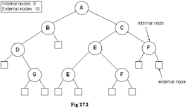
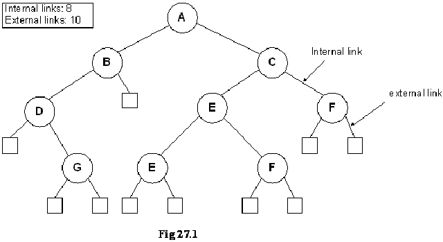
Now, what is a link? As you might already have understood, a link is that line, which we draw between two nodes in a tree. Internally we use pointers in C++ to realize links. In pictorial sketches, however, we use a line to show a link between the two nodes. The property defines, that if you have a binary tree with Nodes, how many links, it will have between the internal nodes (remember, it includes the leaf nodes), and how many links it will have between the external nodes. We have not been showing any links between the external nodes in the diagrams. These are, in fact, null pointers. That means, these are the links, which we will show with the help of the square nodes. Let us see a binary tree, on the basis of which, we will further explore this property. In the following figure, the binary tree is shown again, which, in addition to the normal links between the internal nodes, also contains external nodes as squares and the external links as lines going to those squares.
clip_image002
Now if you count the total number of links in the diagram between internal and external nodes, it will be 2N. Remember, we are talking about links and not nodes. In this tree, we have 9 nodes marked with capital letters, 8 internal links and 10 external links. Adding the both kinds of links, we get 18, which is exactly 2 x 9.
As discussed already that these properties are mathematical theorems and can therefore be proven mathematically. Let us now prove this property as to how do we get 2N links in a binary tree with N internal nodes.
Property
A binary tree with N internal nodes has 2N links, N-1 links to internal nodes and N+1 links to external nodes.
- In every rooted tree, each node, except the root, has a unique parent.
- Every link connects a node to its parents, so there are N-1 links connecting internal nodes.
- Similarly each of the N+1 external nodes has one link to its parents.
- Thus N-1+N+1=2N links.
In the previous lectures, I told you about the important property of the trees, that they contain only one link between the two nodes. I had also shown you some structures, which did not follow this property and I told you, that those were graphs.
Threaded Binary Trees
- In many applications binary tree traversals are carried out repeatedly.
- The overhead of stack operations during recursive calls can be costly.
- The same would true if we use a non-recursive but stack-driven traversal procedure
- It would be useful to modify the tree data structure which represents the binary tree so as to speed up, say, the inorder traversal process: make it "stack-free".
You must be remembering that there were four traversing methods of binary trees: preorder, inorder,
postorder and levelorder. First three preorder, inorder and postorder were implemented using recursion. Those recursive routines were very small, 3 to 4 lines of code and they could be employed to traverse a tree of any size.
We also traversed BST in inorder to retrieve the information in sorted order. We employed stacks in recursive implementations. Although, recursive routines are of few lines but when recursion is in action, recursive stack is formed that contains the function calls. We also explicitly used stack for inorder non-recursive traversal. When the calling pattern of recursive and non-recursive stack based routines were compared, the calling pattern of both of the routines were similar.
Suppose that we have a BST that is traversed again and again for some operations of find or print. Due to lot of recursive operations, the stack size keeps on growing. As a result, the performance is affected. To overcome this performance bottleneck, we can use non-recursive method but stack-driven traversal will again be an issue. The push and pop operations of stack for insertion and retrieval will again take time. So is there a way to do traversal without using a stack neither of implicit function call stack nor explicit. The same idea is presented in the last bullets above that leads to threaded binary trees:
- It would be useful to modify the tree data structure which represents the binary tree so as to speed up, say, the inorder traversal process: make it "stack-free".
The idea in the above statement is to modify the tree data structure to speed up and make it stack-free. Now, we see what kind of modification is required in the binary trees.
- Oddly, most of the pointer fields in our representation of binary trees are NULL!
- Since every node (except the root) is pointed to, there are only N-1 non-NULL pointers out of a possible 2N (for an N node tree), so that N+1 pointers are NULL.
We know that all the leaf node pointers are NULL. Each node of the tree contains the data part, two pointer variables for left and right nodes links. But these pointer variables are used when the node has further child nodes. We know that in a binary tree the total number of links are 2N including both internal and external and the number of NULL pointers is N+1.
clip_image004
In the figure above, the tree is the same as shown in Fig 27.1. The square nodes shown in this figure are external nodes. Thinking in terms of pointers all the pointers of these nodes are NULL or in other words they are available to be used later. We recognize these nodes as leaf nodes. Besides that, what can we achieve using them is going to be covered in Threaded Binary Trees.
- The threaded tree data structure will replace these NULL pointers with pointers to the inorder successor (predecessor) of a node as appropriate.
We are creating a new data structure inside the tree and when the tree will be constructed, it will be called a threaded binary tree. The NULL pointers are replaced by the inorder successor or predecessor. That means while visiting a node, we can tell which nodes will be printed before and after that node.
- We'll need to know whenever formerly NULL pointers have been replaced by non NULL pointers to successor/predecessor nodes, since otherwise there's no way to distinguish those pointers from the customary pointers to children.
This is an important point as we need to modify our previous logic of identifying leaf nodes. Previously the node with left and right nodes as NULL was considered as the leaf node but after this change the leaf node will contain pointers to predecessor and successor. So in order to identify that the pointers has been modified to point to their inorder successor and predecessor, two flags will be required in the node. One flag will be used for successor and other for predecessor. If both the pointers were NULL, left pointer variable will be used to point inorder predecessor, the flag for this will be turned on and the right pointer variable will be used to keep inorder successor and the flag will be turned on once the successor address is assigned.
Adding Threads During Insert
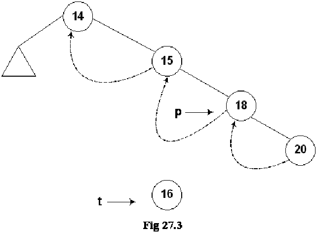
clip_image006
If we print the above tree in inorder we will get the following output:
14 15 18 20
In the above figure, the node 14 contains both left and right links. The left pointer is pointing to a subtree while the right subtree is pointing to the node 15. The node 15’s right link is towards 18 but the left link is NULL but we have indicated it with a rounded dotted line towards 14. This indicates that the left pointer points to the predecessor of the node.
Below is the code snippet for this logic.
t->L = p->L; // copy the thread
t->LTH = thread;
t->R = p; // *p is successor of *t
t->RTH = thread;
p->L = t; // attach the new leaf
p->LTH = child;
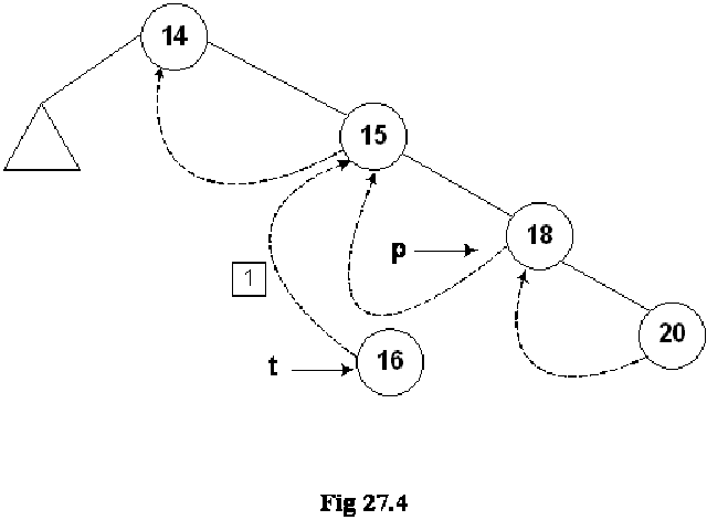
Let’s insert a new node in the tree shown in the above figure. The Fig 27.4 indicates this new insertion.
clip_image008
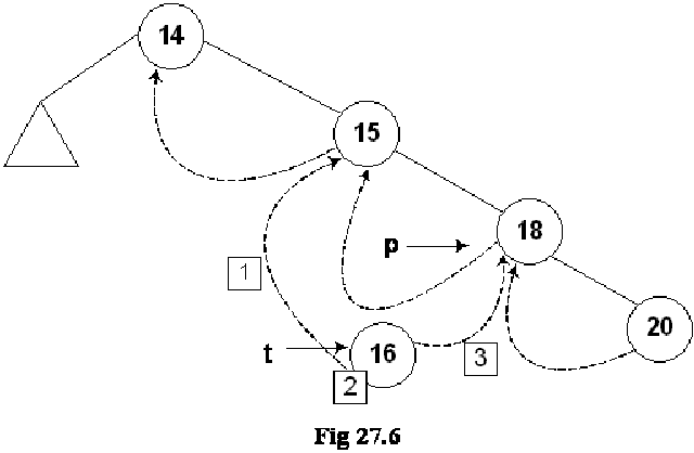
The new node 16 is shown in the tree. The left and right pointers of this new node are NULL. As node 16 has been created, it should be pointed to by some variable. The name of that variable is t. Next, we see the location in the tree where this new node with number 16 can be inserted. Clearly this will be after the node 15 but before node 18. As a first step to insert this node in the tree as the left child of the node 18, we did the following:
1. t->L = p->L; // copy the thread
2. t->LTH = thread;
3. t->R = p; // *p is successor of *t
4. t->RTH = thread;
5. p->L = t; // attach the new leaf
6. p->LTH = child;
As the current predecessor of node 18 is 15. After node 16 will be inserted in the tree, it will become the inorder predecessor of 18, therefore, in the first line of the code t->L = p->L, left pointer of node 18 (pointed to by pointer p) is assigned to the left pointer of node 16 (pointer to by pointer t).
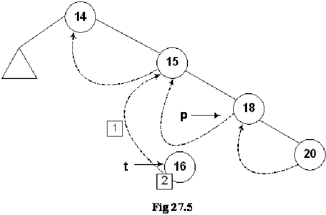
clip_image010
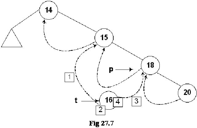
In the next line of code t->LTH = thread, the left flag is assigned a variable thread that is used to indicate that it is on.
clip_image012
In the third line of code, t->R = p, 18 being the successor of node 18, its pointer p is assigned to the right pointer (t->R) of node 16.
clip_image014
Next line, t->RTH = thread contains flag turning on code.
clip_image016
In the next line p->L = t, the node 16 is attached as the left child of the node 18.
clip_image018
The flag is truned on in the last line, p->LTH = child.
If we insert few more nodes in the tree, we have the tree as given below:
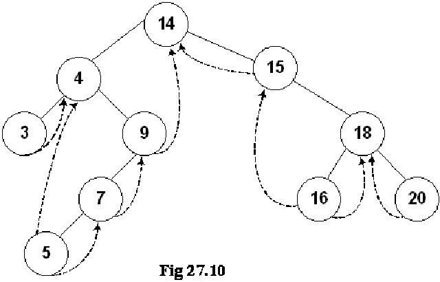
clip_image020
Above given is a BST and you have seen many BSTs before, which are not thread binary trees. Without the threads, it is clear from the figure that there are number of links present in the tree that are NULL. We have converted the NULLs to threads in this tree.
Let’s do inorder non-recursive traversal of the tree. We started at 14 then following the left link came to 4 and after it to 3. If we use recursion then after the call for node 3 is finished (after printing 3), it returns to node 4 call and then 4 is printed using the recursive call stack. Here we will print 3 but will not stop. As we have used threads, we see the right pointer of node 3 that is not NULL and pointing to its successor node 4, we go to 4 and print it. Now which node is inorder successor of node 4. It is node 5.
From node 4, we traversed to right child of it node 9. From node 9, we went to node 7 and then finally node 5. Now, this node 5 is a leaf node. Previously, without using threads, we could identify leaf nodes, whose both pointers left and right were NULL. In this case, using threads, as discussed above, we set the pointers and turn the flags on when a pointer left or right is set to its predecessor or successor. After printing node 5, we traverse its right thread and go to node 7. In this fashion, whole of the tree can be traversed without recursion.
Now, let’s see some code:
TreeNode* nextInorder(TreeNode* p)
{
if(p->RTH == thread)
return(p->R);
else {
p = p->R;
while(p->LTH == child)
p = p->L;
return p;
}
}
Above given is a routine nextInorder, which gives the inorder
successor of a node passed in parameter pointer p. Now what it does is:
If the RTH flag of the p node (the node passed in the parameter) is thread then it will return the node being pointed by the right thread (p->R), which would be its inorder successor. Otherwise, it does the following.
It goes to the right node of p and starts pointing it using the same p pointer. From there it keeps on moving (in a loop fashion) towards the left of the node as long as the statement p->LTH == child is true. After this loop is terminated, the node p is returned.
Next, we see this pictorially.
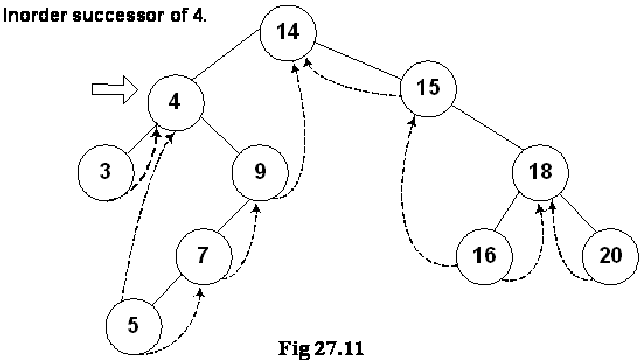
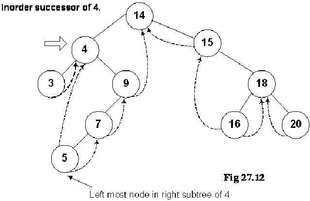
Where is Inorder Successor?
clip_image022
We are at node 4 and want to find its inorder successor. If you remember the delete operation discussed in the previous lecture, where we searched for the inorder successor and found it to be the left-most node in the right subtree of the node.
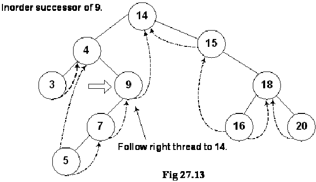
clip_image024
In this figure, the right subtree of 4 is starting from node 9 and ending at node 5. Node 5 is the left most node of it and this is also the inorder successor of node 4. We cannot go to node 5 directly from node 4, we go to node 9 first then node 7 and finally to node 5.
clip_image026
We move from node 9 to node 5 following the normal tree link and not thread. As long as the normal left tree link is there of a node, we have set the LTH flag to child. When we reach at node 5, the left link is a thread and it is indicated with a flag. See the while loop given in the above routine again:
while(p->LTH == child)
p = p->L;
return p;
Inorder Traversal
Now by using this routine, we try to make our inorder traversal procedure that is non-recursive and totally stack free.
If we can get things started correctly, we can simply call nextInorder repeatedly (in a simple loop) and move rapidly around the tree inorder printing node labels (say) - without a stack.
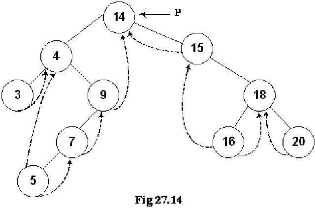
clip_image028
The pointer p is pointing to the root node of the tree. If we start traversing from this node and pass this root node pointer to our routine nexInorder above, it will create a problem.
We see the routine again to see the problem area clearly:
TreeNode* nextInorder(TreeNode* p)
{
if(p->RTH == thread)
return(p->R);
else {
p = p->R;
while(p->LTH == child)
p = p->L;
return p;
}
}
In the first part, it is checking for the RTH flag to be set to thread, which is not the case for the root node. The control will be passed to the else part of the routine. In else part, in the very first step, we are moving towards right of root that is to node 15.
clip_image030
If we call nextInorder with the root of the binary tree, we're going to have some difficulty. The code won't work at all the way we want.
Note that in this tree inorder traversal, the first number we should print is 3 but now we have reached to node 15 and we don’t know how can we reach node 3. This has created a problem. In the lecture, we will make a small change in this routine to cater to this situation i.e. when a root node pointer is passed to it as a parameter. After that change the routine will work properly in case of root node also and it will be non-recursive, stack free routine to traverse the tree.
Inorder traversal in threaded trees
We have introduced the threads in the tree and have written the nextInorder routine. It is sure that the provision of the root can help this routine perform the inorder routine properly. It will go to the left most node before following the threads to find the inorder successors. The code of the routine is given below:
/* The inorder routine for threaded binary tree */
TreeNode* nextInorder(TreeNode* p){
if(p->RTH == thread) return(p->R);
else {
p = p->R;
while(p->LTH == child)
p = p->L;
return p;
}
}
When we apply this routine on the sample tree, it does not work properly because the pointer that points to the node goes in the wrong direction. How can we fix this problem? Let’s review the threaded binary tree again:
clip_image001
In the above figure, we have a binary search tree. Threads are also seen in it. These threads points to the successor and predecessor.
Our nextInoder routine, first of all checks that the right pointer of the node is thread. It means that it does not point to any tree node. In this case, we will return the right pointer of the node as it is pointing to the inorder successor of that node. Otherwise, we will go to some other part. Here we will change the value of pointer p to its right before running a while loops as long as the left pointer is the node. That means the left child is not a thread. We move to the left of the pointer p and keep on doing so till the time the left pointer becomes a thread.
We will pass the root of the tree to the nextInorder routine. The pointer p is pointing to the node 14 i.e. the root node. As the right pointer of the node 14 is not a thread, so the pointer p will move to the node 15 as shown below:
clip_image002[5]
Here we want the inorder traversal. It is obvious from the above figure that 15 is not the first value. The first value should be 3. This means that we have moved in the wrong direction. How this problem can be overcome? We may want to implement some logic that in case of the root node, it is better not to go towards the right side. Rather, the left side movement will be appropriate. If this is not the root node, do as usual. It may lend complexities to our code. Is there any other way to fix it? Here we will use a programming trick to fix it.
We will make this routine as a private member function of the class so other classes do not have access to it. Now what is the trick? We will insert a new node in the tree. With the help of this node, it will be easy to find out whether we are on the root node or not. This way, the pointer p will move in the correct direction.
Let’s see this trick. We will insert an extra node in the binary tree and call it as a dummy node. This is well reflected in the diagram of the tree with the dummy node. We will see where that dummy node has been inserted.
clip_image003
This dummy node has either no value or some dummy value. The left pointer of this node is pointing to the root node of the tree while the right pointer is seen pointing itself i.e. to dummy node. There is no problem in doing all these things. We have put the address of dummy node in its right pointer and pointed the left thread of the left most node towards the dummy node. Similarly the right thread of the right-most node is pointing to the dummy node. Now we have some extra pointers whose help will make the nextInorder routine function properly.
Following is a routine fastInorder that can be in the public interface of the class.
/* This routine will traverse the binary search tree */
void fastInorder(TreeNode* p)
{
while((p=nexInorder(p)) != dummy) cout << p->getInfo();
}
This routine takes a TreeNode as an argument that make it pass through the root of the tree. In the while loop, we are calling the nextInorder routine and pass it p. The pointer returned from this routine is then assigned to p. This is a programming style of C. We are performing two tasks in a single statement i.e. we call the nextInorder by passing it p and the value returned by this routine is saved in p. Then we check that the value returned by the nextInorder routine that is now actually saved in p, is not a dummy node. Then we print the info of the node. This function is called as:
fastInorder(dummy);
We are not passing it the root of the tree but the dummy node. Now we will get the correct values and see in the diagrams below that p is now moving in the right direction. Let’s try to understand this with the help of diagrams.
First of all we call the nextInorder routine passing it the dummy node.
clip_image004[5]
The pointer p is pointing to the dummy node. Now we will check whether the right pointer of this node is not thread. If so, then it is advisable to move the pointer towards the right pointer of the node. Now we will go to the while loop and start moving on the left of the node till the time we get a node with the left pointer as thread. The pointer p will move from dummy to node 14. As the left pointer of node 14 is not thread so p will move to node 4. Again the p will move to node 3. As the left pointer of p is thread, the while loop will finish here. This value will be returned that is pointing to node 3. The node 3 should be printed first of all regarding the inorder traversal. So with the help of our trick, we get the right information.
Now the while loop in the fastInorder will again call the nextInorder routine. We have updated the value of p in the fastInorder that is now pointing to the node 3. This is shown in the figure below:
clip_image005
According to the code, we have to follow the right thread of the node 3 that is pointing to the node 4. Therefore p is now pointing to the node 4. Here 4 is inorder successor of 3. So the pointer p has moved to the correct node for inorder traversal.
As the right pointer of the node 4 is a link, p will move to node 9. Later, we will go on the left of nodes and reach at the node 5. Looking at the tree, we know that the inorder successor of the node 4 is node 5. In the next step, we will get the node 7 and so on. With the help of threads and links, we are successful in getting the correct inorder traversal. No recursive call has been made so far. Therefore stack is not used. This inorder traversal will be faster than the recursive inorder traversal. When other classes use this routine, it will be faster. We have not used any additional memory for this routine. We are using the null links and putting the values of thread in it. This routine is very simple to understand. In the recursive routines, we have to stop the recursion at some condition. Otherwise, it will keep on executing and lead to the aborting of our program.

November 18, 2012

Huffman Encoding

There are other uses of binary trees. One of these is in the compression of data. This is known as Huffman Encoding. Data compression plays a significant role in computer networks. To transmit data to its destination faster, it is necessary to either increase the data rate of the transmission media or simply send less data. The data compression is used in computer networks. To make the computer networks faster, we have two options i.e. one is to somehow increase the data rate of transmission or somehow send the less data. But it does not mean that less information should be sent or transmitted. Information must be complete at any cost.
Suppose you want to send some data to some other computer. We usually compress the file (using winzip) before sending. The receiver of the file decompresses the data before making its use. The other way is to increase the bandwidth. We may want to use the fiber cables or replace the slow modem with a faster one to increase the network speed. This way, we try to change the media of transmission to make the network faster. Now changing the media is the field of electrical or communication engineers. Nowadays, fiber optics is used to increase the transmission rate of data.
With the help of compression utilities, we can compress up to 70% of the data. How can we compress our file without losing the information? Suppose our file is of size 1 Mb and after compression the size will be just 300Kb. If it takes ten minutes to transmit the 1 Mb data, the compressed file will take 3 minutes for its transmission. You have also used the gif images, jpeg images and mpeg movie files. All of these standards are used to compress the data to reduce their transmission time. Compression methods are used for text, images, voice and other types of data.
We will not cover all of these compression algorithms here. You will study about algorithms and compression in the course of algorithm. Here, we will discuss a special compression algorithm that uses binary tree for this purpose. This is very simple and efficient method. This is also used in jpg standard. We use modems to connect to the internet. The modems perform the live data compression. When data comes to the modem, it compresses it and sends to other modem. At different points, compression is automatically performed. Let’s discuss Huffman Encoding algorithm.
Huffman code is method for the compression of standard text documents. It makes use of a binary tree to develop codes of varying lengths for the letters used in the original message. Huffman code is also part of the JPEG image compression scheme. The algorithm was introduced by David Huffman in 1952 as part of a course assignment at MIT.
Now we will see how Huffman Encoding make use of the binary tree. We will take a simple example to understand it. The example is to encode the 33-character phrase:
"traversing threaded binary trees"
In the phrase we have four words including spaces. There is a new line character in the end. The total characters in the phrase are 33 including the space. We have to send this phrase to some other computer. You know that binary codes are used for alphabets and other language characters. For English alphabets, we use ASCII codes. It normally consists of eight bits. We can represent lower case alphabets, upper case alphabets, 0,1,…9 and special symbols like $, ! etc while using ASCII codes. Internally, it consists of eight bits. If you have eight bits, how many different patterns you can be have? You can have 256 different patterns. In English, you have 26 lower case and 26 upper case alphabets. If you have seen the ASCII table, there are some printable characters and some unprintable characters in it. There are some graphic characters also in the ASCII table.
In our example, we have 33 characters. Of these, 29 characters are alphabets, 3 spaces and one new line character. The ASCII code for space is 32 and ASCII code for new line character is 10. The ASCII value for ‘a’ is 95 and the value of A is 65. How many bits we need to send 33 characters? As every character is of 8 bits, therefore for 33 characters, we need 33 * 8 = 264. But the use of Huffman algorithm can help send the same message with only 116 bits. So we can save around 40% using the Huffman algorithm.
Let’s discuss how the Huffman algorithm works. The algorithm is as:
  • List all the letters used, including the "space" character, along with the frequency with which they occur in the message.
  • Consider each of these (character, frequency) pairs to be nodes; they are actually leaf nodes, as we will see.
  • Pick the two nodes with the lowest frequency. If there is a tie, pick randomly amongst those with equal frequencies.
  • Make a new node out of these two, and turn two nodes into its children.
  • This new node is assigned the sum of the frequencies of its children.
  • Continue the process of combining the two nodes of lowest frequency till the time only one node, the root is left.
Let’s apply this algorithm on our sample phrase. In the table below, we have all the characters used in the phrase and their frequencies.
Original text:
traversing threaded binary trees
size: 33 characters (space and newline)

Letters : Frequency
NL : 1
SP : 3
a : 3
b : 1
d : 2
e : 5
g : 1
h : 1


The new line occurs only once and is represented in the above table as NL. Then white space occurs three times. We counted the alphabets that occur in different words. The letter a occurs three times, letter b occurs just once and so on.
Now we will make tree with these alphabets and their frequencies.
clip_image001[4]
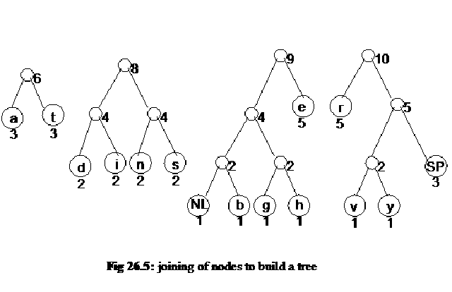
We have created nodes of all the characters and written their frequencies along with the nodes. The letters with less frequency are written little below. We are doing this for the sake of understandings and need not to do this in the programming. Now we will make binary tree with these nodes. We have combined letter v and letter y nodes with a parent node. The frequency of the parent node is 2. This frequency is calculated by the addition of the frequencies of both the children.
In the next step, we will combine the nodes g and h. Then the nodes NL and b are combined. Then the nodes d and i are combined and the frequency of their parent is the combined frequency of d and i i.e. 4. Later, n and s are combined with a parent node. Then we combine nodes a and t and the frequency of their parent is 6. We continue with the combining of the subtree with nodes v and y to the node SP. This way, different nodes are combined together and their combined frequency becomes the frequency of their parent. With the help of this, subtrees are getting connected to each other. Finally, we get a tree with a root node of frequency 33.
clip_image002[4]
We get a binary tree with character nodes. There are different numbers with these nodes that represent the frequency of the character. So far, we have learnt how to make a tree with the letters and their frequency
Huffman encoding is used in data compression. Compression technique is employed while transferring the data. Suppose there is a word-document (text file) that we want to send on the network. If the file is, say, of one MB, there will be a lot of time required to send this file. However, in case of reduction of size by half through compression, the network transmission time also get halved. After this example, it will be quite easy to understand the Hoffman encoding to compress a text file.
We know that Huffman code is a method for the compression of standard text documents. It makes use of a binary tree to develop codes of varying lengths for the letters used in the original message. Huffman code is also a part of the JPEG image compression scheme. David Huffman introduced this algorithm in the year 1952 as part of a course assignment at MIT.
In the previous lecture, we had started discussing a simple example to understand Huffman encoding. In that example, we were encoding the 32-character phrase: "traversing threaded binary trees". If this phrase were sent as a message in a network using standard 8-bit ASCII codes, we would have to send 8*32= 256 bits. However, the Huffman algorithm can help cut down the size of the message to 116 bits.
In the Huffman encoding, following steps are involved:
  1. List all the letters used, including the "space" character, along with the frequency with which they occur in the message.
  2. Consider each of these (character, frequency) pairs as nodes; these are actually leaf nodes, as we will see later.
  3. Pick two nodes with the lowest frequency. If there is a tie, pick randomly amongst those with equal frequencies
  4. Make a new node out of these two and develop two nodes as its children.
  5. This new node is assigned the sum of the frequencies of its children.
  6. Continue the process of combining the two nodes of lowest frequency till the time, only one node, the root, is left.
In the first step, we make a list of all letters (characters) including space and end line character and find out the number of occurrences of each letter/character. For example we ascertain how many times the letter ‘a’ is found in the file and how many times ‘b’ occurs and so on. Thus we find the number of occurrences (i.e. frequency) of each letter in the text file.
In the step 2, we consider the pair (i.e. letter and its frequency) as a node. We will consider these as leaf nodes. Afterwards, we pick two nodes with the lowest frequency in the list. If there are more than one pairs of same frequency, we will choose a pair randomly amongst those with equal frequencies.
Suppose, in a file, the letter ‘a’ occurs 50 times and ‘b’ and ‘c’ five times each. Here, ‘b’ and ‘c’ have the lowest frequency. We will take these two letters as leaf nodes and build the tree from these ones. As fourth step states, we make a new node as the parent of these two nodes. The ‘b’ and ‘c’ are its children. In the fifth step, we assign to this new node the frequency equal to the sum of the frequencies of its children. Thus a three-node tree comes into existence. This is shown in the following figure.
clip_image001
We continue this process of combining the two nodes of lowest frequency till the time, only one node i.e. the root is left.
Now we come back to our example. In this example, there is a text string as written below.
traversing threaded binary trees
The size of this character string is 33 (it includes 3 space characters and one new line character). In the first step, we perform the counting of different characters in the string manually. We do not assign a fake or zero frequency to a letter that is not present in the string. A programmer may be concerned only with the characters/letters that are present in the text. We see that the letters and their frequencies in the above text is as given below.
Character frequency character frequency
NL 1 I 2
SP 3 n 2
A 3 r 5
B 1 s 2
D 2 t 3
E 5 v 3
G 1 y 1
H 1
Table 1: Frequency table
In the second step, we make nodes of these pairs of letters and frequencies. The following figure (fig 26.2) depicts the letters as nodes. We have written the frequency of each letter with the node. The nodes have been categorized with respect to the frequencies for simplicity. We are going to build the tree from downside i.e. from the lowest frequency.
Now according to third step, two nodes of lowest frequency are picked up. We see that nodes NL, b, g, h, v and y have the frequency 1. We randomly choose the nodes v and y. now, as the fourth step, we make a new node and join the leaf nodes v and y to it as its children. We assign the frequency to this new (parent) node equal to the sum of the frequencies of its children i.e. v and y. Thus in the fifth step; the frequency of this new node is 2. We have written no letter in this node as shown in the figure below.
clip_image002
2 is equal to sum
of the frequencies of
the two children nodes.
Now we continue this process with other nodes. Now we join the nodes g and h as children of a new node. The frequency of this node is 2 i.e. the sum of frequencies of g and h. After this, we join the nodes NL and b. This also makes a new node of frequency 2. Thus the nodes having frequency 1 have joined to the respective parent nodes. This process is shown in the following figure (Fig 26.3).
clip_image003
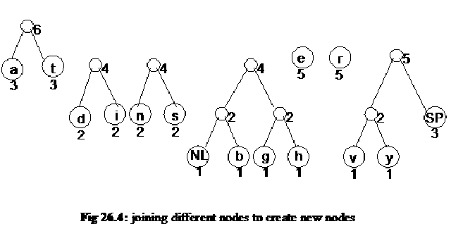
Now we come to the nodes with a frequency 2. Here we join the pair of nodes d and i and also the pair n and s. Resultantly, the two nodes coming into being after joining have the frequency 4. This frequency is the sum of the frequencies of their children. Now, we will bring the nodes, a and t together. The parent node of a and t has the frequency 6 i.e. the sum of a and t. These new nodes are shown in the following figure.
clip_image004
Now we consider these new nodes as inner nodes and build the tree upward towards the root. Now we take the node SP and join it with the node that is the parent of v and y. The resultant node has frequency 5 as the frequencies of its children are 2 and 5 respectively. Now we join these nodes of higher frequencies. In other words, the node r is joined with the newly created node of frequency 5 that is on the left side of node r in the figure 26.5. Thus a new node of frequency 10 is created. We join the node e and the node of frequency 4 on its right side. Resultantly, a new node of frequency 9 comes into existence. Then we join the nodes having frequency 4 and create a new node of frequency 8. The following figure shows the nodes created so far.
clip_image005
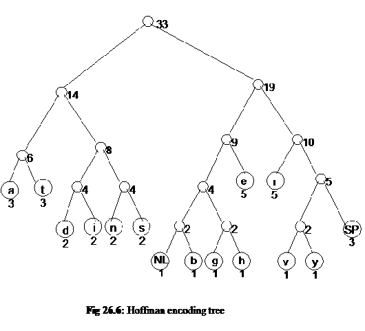
Now we will join the nodes of frequency 6 and 8 to create the node of frequency 14 and join the nodes of frequency of 9 and 10 to develop a new node of frequency of 19. At the end, we make the root node with the frequency 33 and it comprises nodes of frequency 14 and 19. Thus the tree is completed and shown in the following figure.
clip_image006
Now we will perform other steps of Hoffman encoding and develop character-encoding scheme needed for data compression.
To go ahead, we have to do the following steps.
  • Start at the root. Assign 0 to left branch and 1 to the right branch.
  • Repeat the process down the left and right subtrees.
  • To get the code for a character, traverse the tree from the root to the character leaf node and read off the 0 and 1 along the path.
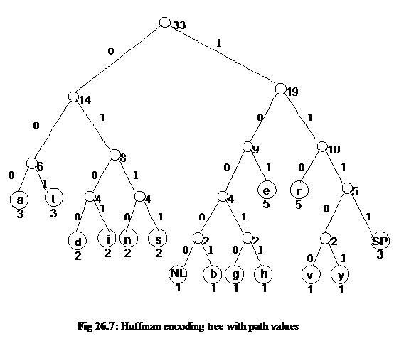
We start from the root node of the tree and assign the value 0 to the left branch and 1 to the right branch. Afterwards, we repeat this value assigning at nodes in left and right subtrees. Thus all the paths have a value 0 or 1 as shown in the following figure. We will develop the code with the help of these path values.
clip_image007clip_image008
In the last step, we get the code for the characters. To get the code for a character, there is need of traversing the tree from the root to the character leaf node and read off the 0 and 1 along the path. We start from the root and go to the letter of leaf node following the edges. 0 and 1 are written down in the order in which they come in this traversal to leaf node. For example, we want the code of letter d. To reach d from the root; we have to go through the nodes of frequency 14. This path has value 0. Here, 0 will be the first digit in the code of d. From 14, we go to node of frequency 8. This link (from 14 to 8) has value 1. Thus the second digit in code is 1. From node of frequency 8, we go to node of frequency 4 to its left side. This side has value 0, meaning that 0 is the third digit of code. From 4, we finally go to d and in this link we get the value 0. Thus we see that to reach at d from the root, we have gone through the branches 0, 1, 0 and 0. Thus, the code of letter d is 0100. Similarly the code of i is 0101. The same way, we find the code for each letter in the tree. The following table shows the letters and their correspondent codes.
character code character code
NL 10000 i 0101
SP 1111 n 0110
a 000 r 110
b 10001 s 0111
d 0100 t 001
e 101 v 11100
g 10010 y 11101
h 10011
Table 2: Hoffman code table
We know that every character is stored in the computer in binary format. Each character has a code, called ASCII code. The ASCII code of a character consists of ones and zeros i.e. it is in binary form. ASCII code is of eight bits. Normally, we remember the decimal value of the characters. For example, letter ‘A’ has decimal value 65. We can easily convert the decimal value into binary one in bit pattern. We need not to remember these values. ASCII value of any character can be found from the ASCII table. The ASCII code of each character is represented in eight bits with different bit patterns.
Here in the example, we assign a code of our own (i.e. Hoffman code) to the letters that are in the message text. This code also consists of ones and zeros. The above table shows the characters and their Hoffman code. Now we come back to the message text from which we developed the tree and assigned codes to the letters in the text.
Look at the table (Table 2) shown above. Here we notice that the code of letters is of variable length. We see that letters with higher frequency have shorter code. There are some codes with a length five that are the codes of NL, b, g, h, v and y. Similarly we see that the letters SP, d, i, n and s have codes of length four. The codes of the remaining letters have length three. If we look at the frequency table (Table 1) of these letters, we see that the letters with some higher frequency like a, e, r, and t, have the code of shorter length, whereas the letters of lower frequency (like NL, b, g, h, v and y) have codes of larger length.
We see in the table of the Hoffman codes of the letters that there will be need of 5, 4 or in some codes only 3 bits to represent a character, whereas in ASCII code, we need 8 bits for each character. Now we replace the letters in the text message with these codes. In the code format i.e. in the form of ones and zeros, the message becomes as under.
Our original message was
traversing threaded binary trees
The encoded form of the message is as under
t r a v e r s i n g t
00111000011100101110011101010110100101111001
100111101010000100101010011111000101010110000
110111011111001110101101011110000


We see that there are only ones and zeros in the code of message. Some letters have been shown with their corresponding code. The first three bits 001 are for letter ‘t’. The next three bits 110 are for letter ‘r’. After this the letter ‘a’ has three bits i.e. 000. Next to it is the letter ‘v’ that has five bits. These bits are 11100 (shaded in the figure). Similarly we have replaced all the letters of the message with their corresponding Hoffman code. The encoded message is shown above.
Let’s compare this Hoffman encoded message with the encoding of message with ASCII code. The ASCII code encoding means that if we have encoded this message with 8 bits per character, the total length of message would be 264. As there are 33 characters, so the total length is 33 x 8 = 264. But in the Hoffman encoded message (written in above table), there are only 120 bits. This number of bits is 54% less than the number of bits in ASCII encoding form. Thus we can send the message with almost half of the original length to a receiver.
Here the Hoffman encoding process comes to an end. In this process, we took a message, did the frequency count of its characters and built a tree from these frequencies. From this tree, we made codes of letters consisting of ones and zeros only. Then with the help of these codes, we did the data compression. In this process we saw that less data is required for the same message.
Now an important thing to be noted is regarding the tree building. We have built the tree with our choices of nodes with same and different frequencies. Now if we have chosen the nodes to join in different way, the tree built would be in a different form. This results in the different Hoffman code for the letters. These will be in ones and zeros but with different pattern. Thus the encoded message would have different codes for the letters. Now the question arises how does the receiver come to know that what code is used for what letter? The answer is very simple that the sender has to tell the receiver that he is using such codes for letters. One way to tackle this problem is that the sender sends the tree built through the use of frequencies, to the receiver to decode the message. The receiver keeps a copy of this tree. Afterwards, when the sender sends a message, the receiver will match it with respect to bit pattern with the tree to see that what letter the sender has sent. The receiver will find the letter for the first 2, 3, 4 or what numbers of bits match to a letter that it has in the tree as the receiver also has a copy of the tree. We know that a tree has a root, inner nodes and leaf node(s). The leaf node is a node whose left and right links is NULL. An inner node has a left or right or both children. Now consider that the receiver has the same tree data structure that the sender used to construct the codes. The sender has sent the message that we have discussed above. The sender sends the 122 bits encoded message to the receiver. The receiver will take the first bit of message and being on the root of the tree, it will decide that on what side this bit will go. If the bit is zero, it will go to the left of the root. However, if the bit is one, it will go to the right side of the root before reaching to the child node. The next bit will go to the next level of the tree to the left or right side depending on zero or one. Thus the traversal will go one level down on receiving a bit. If we (the receiver) are on a path of the tree where the leaf node is at level 6, it cannot reach the leaf node unless the receiver receives 6 bits. We consider the case of letter ‘e’ whose code was of three bits. In this case, we go to the first level by first bit and the second bit takes us to the third level. Finally on reaching the third level with the third bit, we get the leaf node. We know that this node is letter ‘e’ as the sender has sent us (as receiver) the whole tree with the characters in the nodes. Thus after traversing the three bits, the receiver has confirmed that it has received the letter ‘e’. Now on receiving the fourth bit, the receiver will go back to the root and continue to choose the path i.e. on zero it will go to the left and on one it will go to right. This way, it will reach the leaf node. The character at that node will be the next character of the message. The bit pattern that was comprised of following these links in the tree is extracted from the message. On the next bit, the receiver again goes to the root node and the previous procedure is repeated to find the next character. This way, it decodes the whole message.
The compression is very useful technique especially for communication purposes. Suppose that we have to send a file of one Mb. Here each line in the file can be compressed to 50 or 60 percent. Thus the file of one MB will be compressed to half MB and can be sent more easily.
There is one more thing about this tree. When we started to build the tree from leaf nodes i.e. bottom-up build of tree, we saw that there were choices for us to choose any two leaf nodes to join. In our example, we chose them at random. The other way to do it is the priority queue. We have seen the example of bank simulation. There we used a priority queue for the events. We know that in a priority queue, the elements do not follow the FIFO (first in first out) rule. But the elements have their position in the queue with respect to a priority. In the example of bank simulation, in the Event Queue, we remove the element from the queue that was going to occur first in the future. We can use priority queue here in such a way that we put the letters in the queue with respect to their frequencies. We will put and remove letters from the queue with respect to their frequency. In this priority queue, the character with lowest frequency is at the start of the queue. If two characters have the same frequency, these will be one after the other in the queue. The character with the larger frequency will be in the last of the queue. Now we take two frequencies from the queue and join them to make a new node. Suppose that the nodes that we joined have frequency 1 and 2 respectively. So the frequency of the new node will be 3. We put this new node in the queue. It takes its position in the queue with respect to its frequency as we are using the priority queue. It is evident in procedure that we proceed to take two nodes form the queue. These are removed and their parent node goes back to the queue with a new frequency. This procedure goes on till the time the queue is empty. The last node that becomes in the queue in the result of this procedure is the root node. This root node has frequency 33 if we apply this procedure to our previous example.
Let’s talk about some general things related to Hoffman encoding. We use modems to connect to Internet. These modems do the compression. The modem has a compression feature. The modem has a chip that performs the task of compression. When we give a sentence of say 80 characters to the modem to send, the modem makes a Hoffman encoded tree of these characters. Then it will make codes from this tree. We know that there is also a modem on the other end that will decode this message. The sender modem will send the tree structure to the receiver. Now the sender modem will send the data in compressed form. The receiving modem will decode this compressed data by using the Hoffman encoded tree. Now the question arises, will these codes be useful for other messages? In our example message the letter ‘y’ has lower frequency and code of five bits. It may happen that in some messages ‘y’ has higher frequency, needing code of less number of bits. To solve this problem, the modems (sender and receiver) revise the codes after a certain time period or after a particular number of bytes. In this revision, they build a new Hoffman tree and exchange it to use it for communication for the next time period or for the next fixed number of bytes.
There is some other compression techniques/algorithms for compression. The zip routines like winzip and the jpeg, mpeg and other image formatting routines use different algorithms for compression. We will read the compression algorithm in detail in the course of Algorithms.

C program to Read From a File

#include <stdio.h> #include <stdlib.h> void main() {     FILE *fptr;     char filename[15];     char ch;   ...